Experiment of The Month

Fluctuations in the Statistical Determination of a Marble Diameter

The setup:

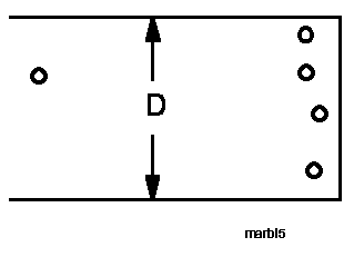
The picture shows a "shooting gallery" consisting of N target marbles and one "shooter" marble. The width of the gallery is D ; the length is not relevant but a meter is typical if the gallery is constructed from meter sticks. N, the number of target marbles, is typically 8 and the width D is typically 60 cm. The precise numbers are not crucial but extremes should be avoided. More about "extremes" later.

Procedure:

The shooter marble is rolled "randomly" down the alleyway. The target marbles are arranged "randomly" on the other end of the alley. On any one roll of the shooter marble there is a one hit or there is a miss. The number of hits by the shooter marble is recorded. The following precautions are important:

1. Randomness is essential - no aiming of the shooter marbles. Do it blind-folded if necessary.
2. Sample the entire width of the alleyway when releasing the shooter. Don't keep rolling the shooter marble from the center of the gallery. Avoid diagonal rolling of the marble across the gallery.
3. Rotate the shooter marble. There will be typically nine marbles in play. The eight targets should be varied and the shooter marble should be varied.
4. The targets must be arranged "randomly but evenly" across the gallery width. Avoid shadowing effects where two or more targets are no longer independent but act as an interacting clump. That is, one or more targets partially shadow other target marbles.
5. If a marble strikes the side of the gallery it is a "no roll". Do it over.
6. Hits on a rebound off the back wall do not count. Multiple hits on the same roll count as just one hit.
7. The alleyway must be level. If marbles roll preferentially to one side then clearly not all portions are randomly sampled.

Preliminary Analysis:

Think of the shooter marble as point-like. Then each target marble presents a target width of 2d where d is the diameter of a marble. The probability of a hit is then p=(2dN)/D.

Suppose that M is the number of rolls resulting in m hits. We can approximate the probability of a hit by p=m/M

and use this empirically determined probability to calculate the diameter of the marble:

d = (mD)/(2MN)

One should note that target marbles cannot really have their centers placed randomly across the full alley width D. A target marble center can be at most within one radius of the side. Consequently. the effective alley width is D-d. For the numbers our lab ( d is nominally 1.5 cm and D= 60 cm) this presents a correction of about 2.5 %. So finally we have:

(Note:) The "edge" effects are actually more numerous and subtle than this simple analysis would indicate. Not only is the full alley width not available for random sampling, but the effective target width of a marble changes near the edge. We will not consider these other complications and Equ. (1) should be considered to be an approximation.

Data:

We take data so as to emphasize statistical fluctuations in the marble diameter. Arrange the students in groups of four or five. A typical lab will have four or five student groups.

1. Each student within a group throws the marble M=10 times, records the number of hits, m, and each student calculates the marble diameter from Equation (1).
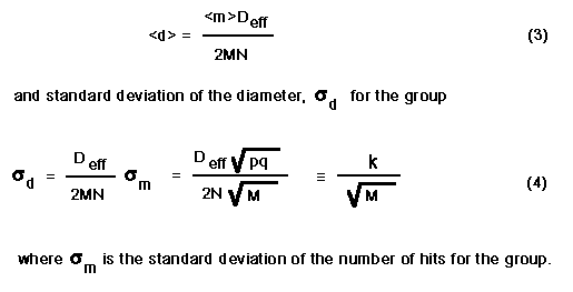
2. Each group then reports three numbers: the average diameter for the group, the standard deviation of the diameter (based on the groups four or five measurements) and the standard deviation of the number of hits for the group.
3. The procedure is repeated for M = 5, 20, 3, 1, 40. Note that mixing up the high and low number of tosses seems to help on randomization and to keep people "out of a rut" when rolling the marble. In the interest of saving time we often "fake" the M= 40 data by taking a run of 20 tries and combining data from a different student group to make forty tries.

One obvious step is to compare the statistically determined marble diameter with a direct measurement of marble diameter. There can be substantial deviations from one marble to the next. The measurement of marble diameter is best carried out by lining up all N+1 marbles, measuring the linear extent of the marbles and dividing by N+1.

Analysis:

The analysis follows from the basics of a binomial distribution. If p is the probability of success, and q=1-p the probability of failure, then out of M attempts, the probability of successes is given by:

Well known results for the binomial distribution give the average number of successes and the standard deviation of the number of successes:

The corresponding values for the marble diameter (now a random variable) are

If marbles of nominal diameter d= 1.50 cm are used with an alley width of 60 cm with N=8 targets then the constant above is numerically given as k= 1.80 cm. These numbers also give a nominal probability of success in any one try of about 0.4 . Extremes in this number should be avoided. If the probability of success is too small or too large, then deviations from the mean are small. If the probability of success is too large, then a large number of marbles is being used and it becomes difficult to avoid shadowing effects. A probability of success on any one trial of approximately 0.4 seems appropriate.

The first issue which arises is "How do we compare our random roll measurements of the marble diameter to the directly measured diameter?" "What quantity do we use as an error estimator?" The answer of course depends on who is doing the comparing.

If we consider individual student measurements of the diameter based on M trials, then we are sampling a population of random variables m with average and standard deviation given by Equ. (2). If one student compares results of M attempts to the direct measurement of the marble diameter then the proper error estimator is given by (sigma sub d) of Equ. (4). However, if the group average is compared (N students each rolling the marble M times), then the proper error estimator is the standard deviation of the mean:

This is, of course just the result of Equ. (4) with MN(students) substituted for M and consequently the standard deviation result for MN(students) measurements. This demonstrates a justification for the square root factor which often mysteriously appears when converting a standard deviation to a standard deviation of the mean.

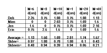
Below are some actual student data of a group of four. The direct measurement of the marble diameter gave a result of 1.43 cm. A number of comparisons can be made using this data. Individual students may compare their results with the direct measurement of marble diameter. The relevant error estimator here is the standard deviation.

Alternatively, the group may compare their statistical diameters for any one M using the standard deviation of the mean.

For example, the direct measurement of 1.43 cm does not fall within the 95% confidence interval (two standard deviations of the mean) for the group data with M=20 throws. The same is true (for M=20 throws) of the individual statistical measurements using not the standard deviation of the mean but rather the standard deviation. M=20 throws seems to have been rather anomalous in this regard for the group.

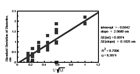
The second part of the analysis is a test of Equ. (4). Graph the standard deviation (sigma sub d) versus 1/(root(M)). For each M, there are four or five values of (sigma sub d): one for each student group. The predictions of Equ. (4) are three fold:

1. the graph is a straight line
2. the graph has zero intercept
3. the (nominal) slope of the graph is 1.80 cm.

Below are some actual student data with a Least Squares Fit analysis. In this particular class there were six groups of four students each. We note that although there is quite bit of scatter, the slope (denoted ao) and intercept (a1) are consistent with the predicted values when the 95% confidence interval is considered. (The 95% intervals are not listed on the chart. S95(ao) =.20 cm and S95(a1) = .37cm.) The scatter of the standard deviation of the diameter is also interesting.

We would expect the range of the standard deviation to go as 1/{4th root of M}. Therefore the data should become "tighter" (but slowly) as M is increased. This effect is probably apparent if we ignore the M=1 data. The sampling numbers are just too small, however, for an unambiguous determination.

We note one final result from our table of data. The group of four had 136 hits out of a total of 316 tries for the entire lab. This corresponds to a probability of success p=0.43 with a corresponding marble diameter given by Equ. (1) of d=1.50cm . The standard deviation on this result is given by Equ. (4) as 0.10cm . Therefore the statistical result, although high, is within two standard deviations (the 95% confidence interval) of the direct measurement. These results hare historically typical of this lab. Statistically determined diameters tend to be larger than the direct measurement although usually within a standard deviation or two of the direct measurement. A number of factors may account for this effect. There are, for example, edge effects which have not been adequately treated and which enter into a calculation of D(effective). It also appears that not all sections of the alley are equally sampled. Marbles rolled near the edge of the alley have a greater probability of hitting the side and are counted "no rolls". It also appears that despite their best efforts, the students on occasion "aim" the marbles.

The edge effects can be completely eliminated by using a circular geometry. The target marbles are arranged "randomly" in a circle with the shooter marble at the center. The shooter is then rolled outward randomly sampling the entire angular extent of the circle.

Back to Main Page of  Marble Scattering Experiment