Experiment of The Month

The MU Physics Department does not claim that we invented these labs. Actually, the origin of these labs are currently unknown to us. Our labs do not have written instructions. In keeping with this spirit, the description given here will be brief and general. The intent is that each performance of the lab will be unique; in each nature will reveal a slightly different face to the observer.

This month we describe a series of three laboratories which are taught in our Physics 103 course. This course is designed for students whose majors are in fields other than the sciences. For example, this year we have the first students in Phy 103 who have elected the science emphasis in their training to be elementary education teachers.

This class has a certain luxury, compared to the courses taken by science majors: While the other courses must deliver a fairly well-defined problem-solving skills, Physics 103 is intended to communicate (by example) the general idea of what it is like to do science. This course can afford to linger on important ideas, and savor the physics.

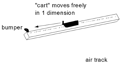
We use "carts" which ride on a track, from which air is blown through many small holes. The cart floats on the air, and can move along the track with almost no friction. The tracks are 2 meters long, and are marked at 1 mm intervals along the length.

A sketch is shown below:

For the first exercise, students use a stop watch program (written by Dr. Miziumski) to measure and record the time at which the cart passes each of 5 points marked on the track, about 20 cm apart. They give the cart a gentle push, and mark the times as the cart travels to the end of the track, bounces on a bumper spring there, and returns to its starting point.

Using a spread sheet (currently Excel), students plot position versus time. The graph shows a "V" shape, with two linear regions; one with positive slope and one with negative slope. This is the pattern for the first exercise. The change in slope when the cart hits the bumper is the sign that the velocity is not constant.

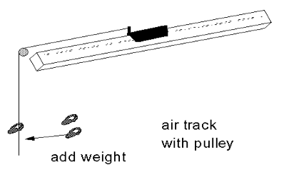
In the second and third exercises, a string is tied to one end of the cart, and passed over a pulley at the end of the track, as sketched below.

The string is weighted with small clips. The cart is released, and timing starts when it bounces from the bumper (not shown) at the end with the pulley, so that students can time it through an entire round trip under the influence of the weights. The graph of position versus time produces a pattern which is harder to describe because the slope (therefore the velocity) is not constant in any region of the graph.

As a "lucky guess," we use the spreadsheet to calculate the average velocity for adjacent points in the data set and plot this velocity versus time, discovering that the pattern is simpler; a straight line. We draw a straight line through the points on the graph and calculate the slope of the line (that is, the acceleration).

We repeat the measurements for 1,2,3,4, and 5 clips on the string. Then we plot the acceleration versus the number of clips and discover a new pattern, which will be used in future to develop the idea of Newton's second law.