Experiment of The Month

Magnetic Fields Varying as an Inverse Cube

Magnetic fields are generally produced by magnetic dipoles, using either permanent magnets or current-carrying loops of wire. This is different from the usual method of producing an electric field, using electric charges (or "monopoles"). For both monopoles and dipoles, the field strength decreases as the distance from the source increases.

For point electric charges, the electric field strength follows Coulomb's law: It is proportional to R ^-2, that is, notation , often called the inverse square law.

For electric dipoles, the field strength decreases more rapidly with distance; as R ^-3 .

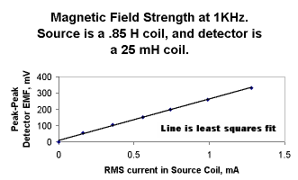
Magnetic monopoles have never been observed. Instead, the basic source of magnetic field seems to have the properties of a magnetic dipole. That assertion is explored in this month's laboratory

We present two versions; a simple demonstration which ignores important details and is quickly done, and a complete exercise which includes the details of the real coil which produces the field. The complete exercise shows in microcosm how physics works: Measurements are analyzed using theory and the analysis is used to predict the results of new measurements.

The MU Physics 232 Experiment

A more complete experiment is done in our Physics 232 laboratories. A large coil is used as the source, and the magnetic field at the center of the coil is calculated from the dimensions of the coil and the current. The detector is once again a 25mH coil, but in this exercise its axis lies on the axis of the large coil. R is now measured along this axis as the detector moves away from the center of the coil.

The EMF induced in the 25mH detector coil is determined by the time derivative of the magnetic field. This magnetic field is calculated from the current through large coil and the geometry of the large coil. The induced EMF in the detector is finally calculated as a function of the current in the large coil.

The current in the source coil is the original measurement. The analysis using electromagnetic theory predicts the nature of the second measurement; the EMF across the 25mH detector coil. This experiment focuses on the distance dependence of that relation.

To keep that focus, uncertainties due to measurements of coil geometry are corrected with an intermediate "calibration" measurement. The detector EMF is measured with R=0, as a function of drive current through the large coil. A plot (at the right) of EMF versus drive current gives a straight line whose slope, K, is the calibration constant. This constant K is used in the formula for induced EMF, to reduce uncertainties due to the geometry of both the detector and the source coil. For the graph shown, the K was 253 mV/mA, with a standard deviation of 5.

The expected detector signal is notation

Where notation is the rms current in the source coil, is the average of the inner and outer coil radii of the source coil, 2l is the coil length, is the measured calibration constant, and is the peak-to-peak induced EMF in the detector coil.

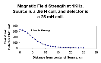
The results of student measurements are shown in two graphs at the right. In this exercise, the frequency was 1KHz, and the detector moved along the axis of the large source coil. In the direct plot, the line is the predicted detector signal, based on the formula above. The agreement with the data points is remarkably good.

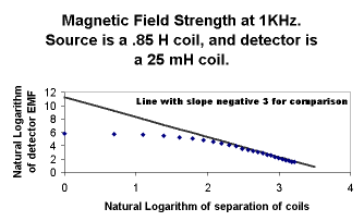
In the "log-log" plot, for large distances, the data are seen to approach the R ^-3 line that is drawn in. (That line is for reference only. Its equation is y=-3x+11.3 .)

When fit to a straight line, the last 10 data points on the log-log graph have a slope of 2.88 with a standard deviation of .05. Both observations are near agreement with the R ^-3 dependence on distance (in the limit as R becomes large) that is predicted by the formula

notation .

A low pass filter improves our signal to noise ratio

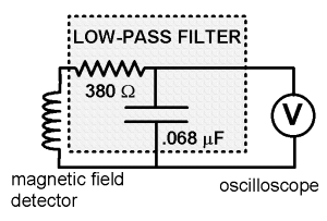
Because of extensive high frequency noise in the Millersville Physics laboratories, it was helpful to use a low pass filter in taking data. This allows us to measure with confidence at larger values of R, where the signal is much reduced. A sketch of the filter, as connected to the detector coil and the oscilloscope, is shown at the right. This filter was used to take the demonstration data with two 25mH coils.